


Linear Regression - My ML Learning Journey 001
Introduction
Hi guys, welcome to my blog! I am Sivvie, it is an honour to meet you here! In this blog post I will share my process and learning journey to submit my first Kaggle entry ever, on topic of Linear Regression from Machine Learning. It is not a tutorial as I do not possessed such knowledge, I merely wanted to record down my learning process towards this brand new topic!
The Kaggle competition that I picked is the Beginner Competition which is right over here: House Prices - Advanced Regression Techniques | Kaggle
After enters the competition and downloaded the CSV data file to my local, here it started 😆
Import Data
First of all I imported the basics into my local Jupyter Notebook.
import pandas as pd # For Read CSV File
import matplotlib.pyplot as plt # For Data Visualization
import seaborn as sns # For Data Visualization
import numpy as np # For Math Operation
These are the packages that first came to my mind when I started:
- pandas - For reading the CSV data file
- matplotlib.pyplot - For data visualization such as bar graphs or scatter plot
- seaborn - For data visualization such as bar plot
- numpy - For mathematics operation etc.
If there is error when import the package, please make sure to
pip installthose packages into your local
After that, I am ready to take a look into the data by
train_data = pd.read_csv('local_path\\train.csv')
test_data = pd.read_csv('local_path\\test.csv')
train_data.head()
Run the cell and the .head() method gave me the first 5 rows of the data, which looks like this:
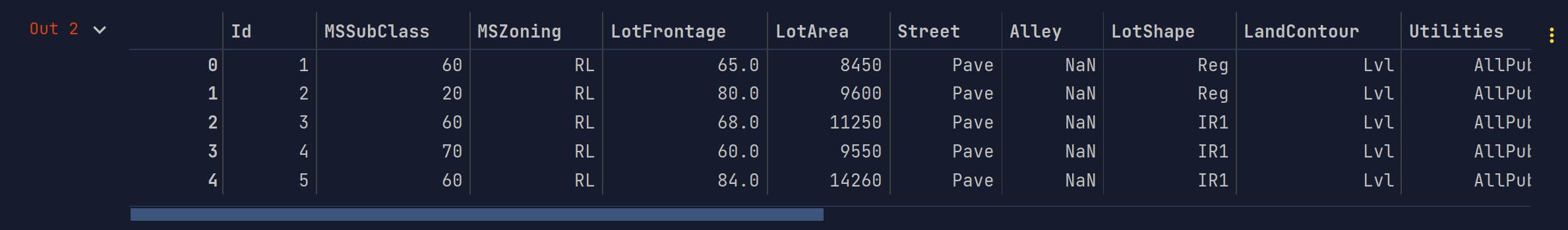
Run another cell with train_data.shape will gave me the shape of the data which looks like this: (1460, 81). And this tells me that the data had 81 columns and 1460 rows. Which I interpreted as having 79 features after excluding Id and SalePrice as the output.
Data Visualization
Then, I want to see how the SalePrice looks like in a histogram, so I plotted them using below:
plt.hist(train_data.SalePrice, color='blue')
plt.show()
It shows something like this:
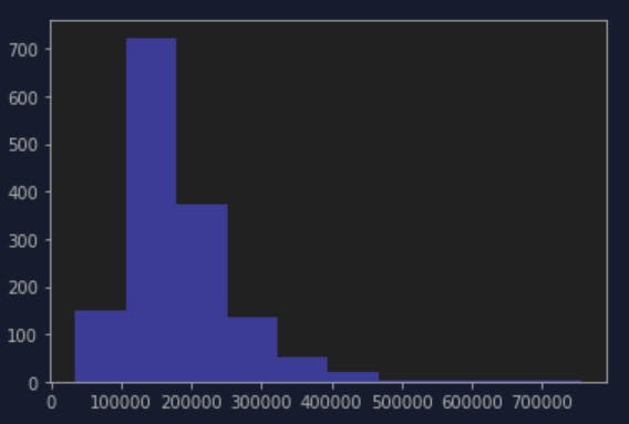
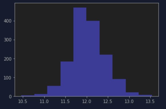
So most of the SalePrice falls about $150000-200000, I also learned a trick to np.log() them to prevent skewed distribution, this graph does not look skewed to me but when I try it, I think it does look better distributed? Like a normal distribution.
plt.hist(np.log(train_data.SalePrice), color='blue')
plt.show()
Next, I think I want to find which feature affected the output the most, so I run below cell with the code
corr = train_data.corr()
print(corr['SalePrice'].sort_values(ascending=False))
And this gave me something like this (I only showcase those have correlation above 0.5 here):
| Feature | Correlation |
| SalePrice | 1.000000 |
| OverallQual | 0.790982 |
| GrLivArea | 0.708624 |
| GarageCars | 0.640409 |
| GarageArea | 0.623431 |
| TotalBsmtSF | 0.613581 |
| 1stFlrSF | 0.605852 |
| FullBath | 0.560664 |
| TotRmsAbvGrd | 0.533723 |
| YearBuilt | 0.522897 |
| YearRemodAdd | 0.507101 |
Now I know the most affected feature is OverallQual followed by GrLiveArea and GarageCars.
If I plotted them into graphs, it looks like this:
overall_quality = train_data.pivot_table(index='OverallQual', values='SalePrice')
overall_quality.plot(kind='bar', color='green')
plt.xlabel('Overall Quality')
plt.ylabel('Sale Price')
plt.xticks(rotation=0)
plt.show()
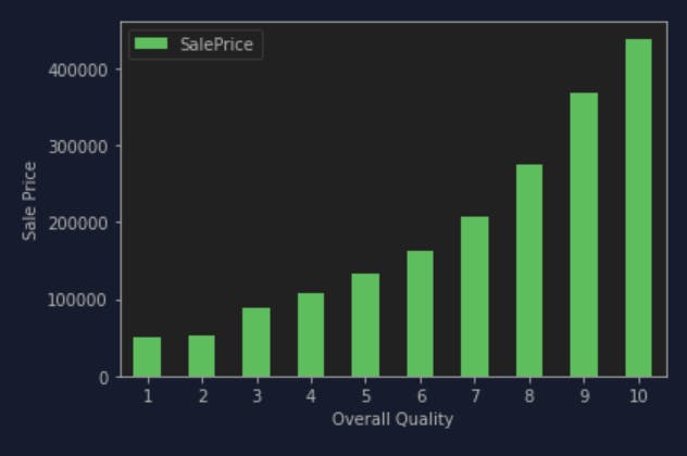
This shows very clear that with the higher overall quality of the house, the higher the sales price. I thought the same will happen to GrLiveArea but it is not quite what I think. When I applied the same code to GrLiveArea it gave me something like this:
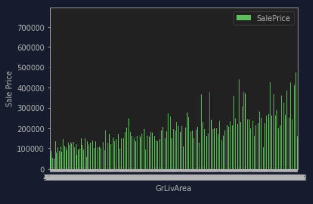
Which is not quite consistent as OverallQual, so I look around the internet and then decides to try out scatter plot with below code cell:
plt.scatter(x=train_data['GrLivArea'], y=train_data['SalePrice'])
plt.ylabel('Sale Price')
plt.xlabel('GrLiveArea')
plt.show()
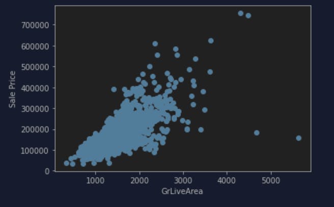
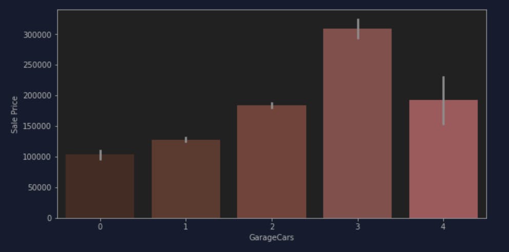
This gave a much better insight on where are most of the ground living area falls in the Sale Price with some outliers. So I probably have to do something with the outliers later. Now I decide to continue with the third feature, which is a discrete value feature so I figured I probably could not plot using the bar graph or scatter plot like the other two features. So for GarageCars I used something called barplot:
plt.figure(figsize=(10,5))
sns.barplot(x=train_data['GarageCars'],y=train_data['SalePrice'],palette='Reds')
plt.ylabel('Sale Price')
plt.show()
I tried for a couple more feature while toying around both matplotlib and seaborn for Data Visualization so that it gave me insights on how is the relationship between features and the ultimate output - Sale Price. I also found some feature have NaN value which needs to be eliminated.
Data Pre-Processing
Next step is to eliminate the NaN value from the data set, so I run below code to check NaN value for every feature:
train_data.isna().sum().sort_values(ascending=False)
| Feature | Number of NaN value |
| PoolQC | 1453 |
| MiscFeature | 1406 |
| Alley | 1369 |
| Fence | 1179 |
| FireplaceQu | 690 |
| LotFrontage | 259 |
| GarageYrBlt | 81 |
| GarageCond | 81 |
| GarageType | 81 |
| GarageFinish | 81 |
| GarageQual | 81 |
| BsmtFinType2 | 38 |
| BsmtExposure | 38 |
| BsmtQual | 37 |
| BsmtCond | 37 |
| BsmtFinType1 | 37 |
| MasVnrArea | 8 |
| MasVnrType | 8 |
These looks a lot of NaN value to me, so again I look around to search for good ways to eliminate the NaN, and I went for this to try out:
train_data = train_data.select_dtypes(include=[np.number]).interpolate().dropna()
train_data.isna().sum().sort_values(ascending=False)
The table is now all showing 0 so I presumed the NaN value has been eliminated. Next step for me is to eliminate the outliers. Again I searched around the internet, and I went for IsolationForest which seems interesting.
from sklearn.ensemble import IsolationForest

isolation_forest = IsolationForest(contamination=0.1)
isolated_result = isolation_forest.fit_predict(train_data)

is_it_outlier = isolated_result != -1
train_data = train_data[is_it_outlier]
Model Training
I guess I can start to prepare for model training now! First of all I defined the X and y of it, which in this case y shall be the Sale Price and X shall be the features but excluded the output and the Id. I defined y as the log of SalePrice to scale better I guess:
y = np.log(train_data.SalePrice)
X = train_data.drop(['SalePrice', 'Id'], axis=1)
Then I use something called train_test_split from scikit-learn to separate the training data into two part for train and test (70% for train and 30% for test):
from sklearn.model_selection import train_test_split
X_train, X_test, y_train, y_test = train_test_split(X, y, random_state=42, test_size=0.3)
Now I have two sets of data for train and test for both X and y, let's train it with the LinearRegression model!
from sklearn import linear_model
from sklearn.metrics import mean_squared_error

regressor = linear_model.LinearRegression()
model = regressor.fit(X_train, y_train)
After I have the trained model, next is to evaluate the performance of the model by using test data
Model Evaluation
I used the R^2 value and Mean Squared Error value as the evaluation value as R-squared value explains how well the model fits the data (the higher the number the better between 0 and 1), and mean squared error value explains the loss function (the lower the number the better between 0 and 1).
print(f"The R^2 value is {model.score(X_test, y_test)}")
predictions = model.predict(X_test)
print(f"The MSE value is {mean_squared_error(y_test, predictions)}")
The result gave me:
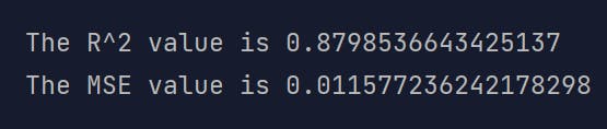
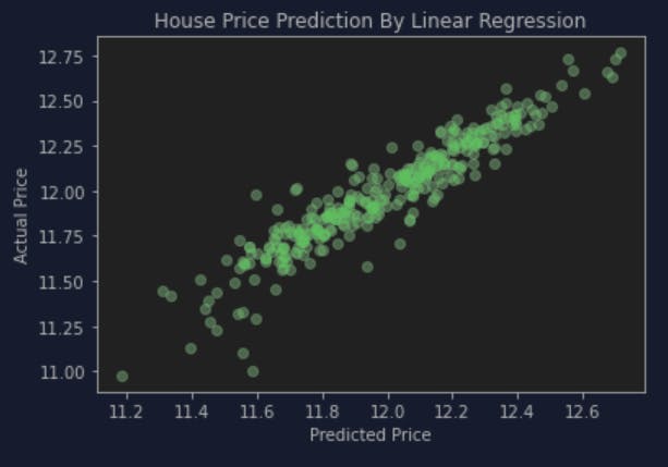
Which is not considered very good I guess but as my first try I felt... pretty satisfied? So I decide to go for this first without any further tweaks. I also plotted a scatter plot to try and see how is the predictions performed:
actual = y_test
plt.scatter(predictions, actual, alpha=0.5, color='g')
plt.xlabel('Predicted Price')
plt.ylabel('Actual Price')
plt.title('House Price Prediction By Linear Regression')
plt.show()
Conclusion
Voila! I think I finished my first try on Linear Regression problem! I then make a submission to Kaggle after creating the output of the test_data for the submission. I placed in about middle ground so I guess there are much to improve. While looked back the code I also noticed in the end I probably only train the model with continuous value feature, maybe next time for improvement I can add in the discrete value feature, which is something new to learn!
Thank you for reading, and if you have any suggestion for the improvement of this practice please do not hesitate to comment! I have a lot to learn and I hope I could improve more and more with the practices!